Any experiment that involves later statistical inference requires a sample size calculation done BEFORE such an experiment starts. A/B testing is no exception. Calculating the minimum number of visitors required for an AB test prior to starting prevents us from running the test for a smaller sample size, thus having an “underpowered” test.
In every AB test, we formulate the null hypothesis which is that the two conversion rates for the control design ([latex]{ \varrho}_{ c }[/latex]) and the new tested design ([latex]{ \varrho}_{ n }[/latex]) are equal:
[latex]{H}_{0 }:{ \varrho}_{ c }={ {\varrho } }_{ n }[/latex]
The null hypothesis is tested against the alternative hypothesis which is that the two conversion rates are not equal:
[latex]{H}_{0 }:{ \varrho}_{ c }\neq { {\varrho } }_{ n }[/latex]
Before we start running the experiment, we establish three main criteria:
- The significance level for the experiment: A 5% significance level means that if you declare a winner in your AB test (reject the null hypothesis), then you have a 95% chance that you are correct in doing so. It also means that you have significant result difference between the control and the variation with a 95% “confidence.” This threshold is, of course, an arbitrary one and one chooses it when making the design of an experiment.
- Minimum detectable effect: The desired relevant difference between the rates you would like to discover
- The test power: the probability of detecting the difference between the original rate and the variant conversion rates.
Using the statistical analysis of the results, you might reject or not reject the null hypothesis. Rejecting the null hypothesis means your data shows a statistically significant difference between the two conversion rates.

Not rejecting the null hypothesis means one of three things:
- There is no difference between the two conversion rates of the control and the variation (they are EXACTLY the same!)
- The difference between the two conversion rates is too small to be relevant
- There is a difference between the two conversion rates but you don’t have enough sample size (power) to detect it.
The first case is very rare since the two conversion rates are usually different. The second case is ok since we are not interested in the difference which is less than the threshold we established for the experiment (like 0.01%).
The worst case scenario is the third one. You are not able to detect a difference between the two conversion rates although it exists. Because of the data, you are completely unaware of it. To prevent this problem from happening, you need to calculate the sample size of your experiment before conducting it.
It is important to remember that there is a difference between the population conversion rates and the sample size conversion observed rates r. The population conversion rate is the conversion rate for the control for all visitors that will come to the page. The sample conversion rate is the control conversion rate while conducting the test.
We use the sample conversion rate to draw conclusions about the population conversion rate. This is how the statistics work: you draw conclusions from the population based on what you see for your sample.
Making a mistake in your analysis based on faulty data (point 3) will impact the decisions you make for the population
Type II errors occur when are not able to reject the hypothesis that should be rejected. With type I errors, you might reject the hypothesis that should NOT be rejected concluding that there is a significant difference between the tested rates when in fact it isn’t.
These two situations are illustrated below:
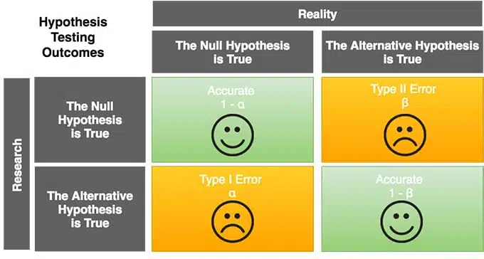
You avoid both of these errors when calculating your sample size.
- To avoid type I errors, you specify a significance level when calculating the sample size.
- To avoid type II errors, you set the power at 0.8 or 0.9 if possible when calculating your sample size, making sure that the sample size is large enough.
How to calculate the sample size for an A/B test?
For no-math-scared readers, I will provide an example of such a calculation later in the post.
The formula for calculating the sample size is pretty complicated so better ask the statistician to do it. There are of course several available online calculators that you can you use as well.
When calculating the sample size, you will need to specify the significance level, power and the desired relevant difference between the rates you would like to discover.
A note on the MDE: I see some people struggle with the concept of MDE when it comes to AB testing. You should remember that this term was created before AB testing as we know it now. Think of an MDE in terms of medical testing. If a new drug produces 10% improvement, it might not be worth the investment. Thus, the MDE is asking the question of what is the minimum improvement for the test to be worthwhile.
The following are some common questions I hear about sample size calculations.
Why does sample size matters in A/B testing?
Sample size matters in A/B testing because it determines the accuracy and reliability of the test results. A small sample size may not be representative of the larger population, and the results may not be statistically significant.
Conversely, a large sample size may increase the accuracy and reliability of the results, but may also increase the time and cost required for the test. Determining the appropriate sample size is critical to ensure that the test results are valid and can be used to make informed decisions about website optimization.
What is a good sample size for an A/B test?
The appropriate sample size for an A/B test depends on several factors, such as the expected effect size, significance level, power, and baseline conversion rate. As a general rule of thumb, a larger sample size is typically better for A/B testing because it increases the accuracy and reliability of the results. However, a larger sample size may also increase the time and cost required for the test.
It is difficult to provide a specific number for a “good” sample size for an A/B test because it depends on the specific context and goals of the test. However, some industry experts suggest a minimum sample size of 100 conversions per variation to ensure statistical significance.
In general, it is recommended to consult with a statistician or use online calculators or statistical software to determine the appropriate sample size for your A/B test based on your specific goals and constraints.
What if you didn’t calculate your sample size? Can I do it after I started the test?

YES! You can calculate the sample size after you started the test. I would not recommend it as a matter of best practice. It is important to remember that all of these statistical constructs are created to ensure your test analysis is done correctly. The problem with not calculating the test size is that you might you stop your test too early because you think it shows significant results while in reality you still did not collect enough data.
If you choose to follow this approach, then do not stop your test unless you made sure that the number of visitors in the test exceeds the minimum required sample size.
What if I collect more data than the sample size called for. For example, if the sample size calls for 1,000 visitors but I go ahead and collect 10,000 – is there a downside to that?
No, there is no downside to this. You just have more power to detect the difference that you assumed was relevant for the test. It might then happen that you conclude that the difference that you observe in rates is significant but it is very small so it will be not relevant for your AB test. It’s like they say “Everything is significant. It’s just a matter of your sample size”.
Related Video:
When sample size calculation fails
It may happen that the standard approaches for sample size calculation fail. This is the case when you can make certain assumptions about the user’s behavior, for example about the sample homogeneity.
One of our clients is a large e-commerce website that receives millions of visitors on daily basis. The last step of the check has an 80% conversion rate. If they conduct an A/B test with a 95% confidence and a 10% MDE, the required sample will be 263 visitors per variation.
It will take about 4 hours to collect the required sample size.
The problem is that these 263 visitors will not be a truly random sample for all visitors in a single day, let alone for a week. For example, different times of day have different conversion rates. Different days of the week have different conversion rates. So running a test Sunday morning is different than running the same test Monday at 10 pm.
How do we consolidate the sample size calculation with what we know about visitor behavior?
This is actually a question about the conversion rate variability. The smaller the variability, the more homogenized your sample is and less sample that you need. The bigger the variability, the more sample you need because of the less exact estimation of the rates. Sometimes you cannot make a sample as homogenous as you would like, such as our client’s example. In that case, a perfect way to calculate a sample size is via simulation methods. They require some more coding and an expert help but in the end, the calculated sample takes into account the real nature of the experiment.
What about recalculating a sample size?

Research studies show that under some conditions the type I error rate is preserved under sample size adjustable schemes that permit a raise. Broberg states that:
“Raising the sample size when the result looks promising, where the definition of promising depends on the amount of knowledge gathered so far, guarantees the protection of the type I error rate”.
What if my website or campaign does not receive enough visitors to match the required A/B test sample size?
When calculating the sample size you usually choose a power level for your experiment at 0.8 or 0.9 (or even more) based on your requirements. You also chose a minimal desired effect. Your experiment is therefore designed to have 0.8 or 0.9 probability of detecting a minimal relevant difference that you have chosen.
Let’s say that based on your inputs, the calculations show that you need a minimum of 10,000 visitors but I can only get 5,000 visitors.
What should you do?
The sample size calculations are impacted by the significance level, power, and minimum detectable effect. Think of them as 4 factors in a formula. You can use any three of them to calculate the fourth unknown one. So, if you already know that you have a small sample size, then evaluate the other three factors: significance level, power, and minimum detectable effect. We always test for the same significance level. The minimum detectable effect is also typically fixed.
Thus, the unknown factor in our calculations is the test power.
You should calculate a power of your experiment to see how much the smaller sample size affects the probability of discovering the difference you would like to detect.
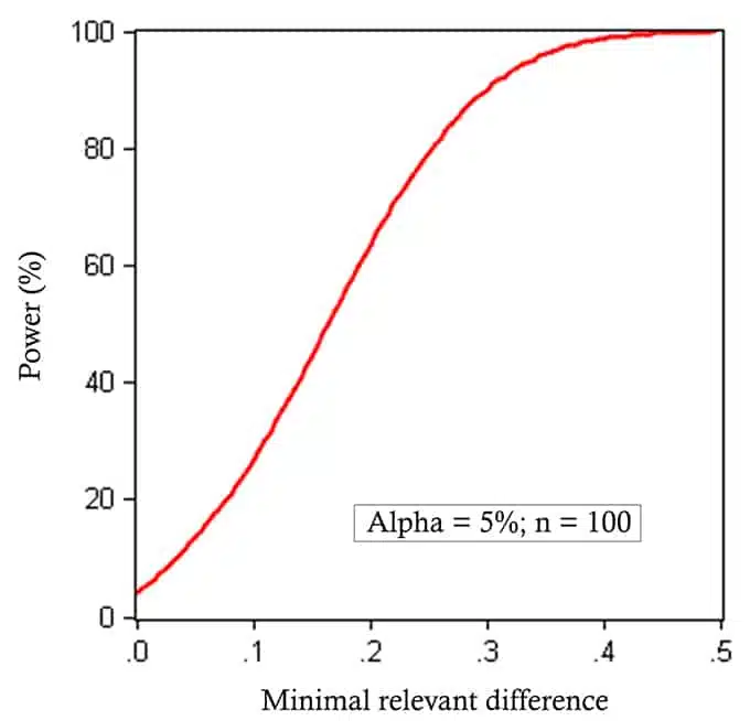
You might also increase the minimum detectable effect since you will have a better chance to detect it with your smaller sample size. If you choose to increase the MDE, then, you should ensure that the power of your experiment is at least 0.8 at least.
The best approach is to create a graph of power depending on the minimum detectable effect like the one below:
You can also relax other assumptions. For example, increasing a significance level leads to gaining some power too:
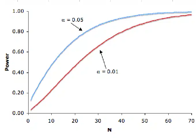
Of course, there is no free lunch and increasing the significance level you allow for a greater probability of type I error.
Early stopping of an AB test
It is very common in medical trials that you stop a study early if the researchers observe that the new drug is obviously better than the standard one. This is called stopping for efficacy. Stopping early in such case saves money, time and patients who are in the control group can switch to the alternative treatment.
Sometimes the clinical trials are stopped because they are not likely to show the significant effect. That is called stopping for futility.
In the “Interim Analysis: The alpha spending function approach,” Authors DeMets DL and Lan KK, state:
It is “either because of slower than expected accrual, a lower than expected event rate, limited funds, or new evidence discounting the likelihood of a beneficial effect or increased likelihood of harm”[1].
This early stopping procedure is based on so-called “interim looks” or “interim analysis” and it must be planned in advance. So, in case you want to stop your AB test early for efficacy or futility, then the sample size must be adjusted to the planned interim analysis.
There can be more than one interim look to analyze the collected data, but you must also plan the number of interim looks in advance. These methods are called “sequential methods,” and they are borrowed from the medicine and used also in other areas of research such as A/B testing. Historically, these concepts originated from the era of World War II, when sequential methods were developed for the acceptance sampling of manufactured products.
The sequential methods are derived in such a way that at each interim analysis, the study may be stopped if the significance level is very low. For example, an early stopping rule for an experiment with 5 interim analyses may stop the trial:
- If the first analysis was significant at the 0.00001 level (99.9999% confidence)
- If the second analysis was significant at the 0.0001 level (99.99% confidence)
- If the third analysis was significant at the 0.008 level (99.2% confidence)
- If the fourth analysis was significant at the 0.023 level (97.7% confidence)
- If the fifth analysis was significant at the 0.041 level (95.9% confidence)
This means that when we make a first planned interim look analysis we compare the difference between the conversion rates and reject the null hypothesis if the p-value is less than 0.00001. P-value is produced by the statistical software and it is a minimal significance level at which we can reject the null hypothesis.
If in the first interim analysis p-value is greater than 0.00001 we continue the experiment until the second interim analysis. Then we make again the test and we reject the null hypothesis (stop experiment) if the p-value is less than 0.001. If the p-value is greater than 0.001 than we continue until the third interim look and so on.

As you can see, it is very unlikely that we stop the experiment after the first interim analysis but if we are lucky and the true difference between the rates is really higher than we expected that it may happen and we can stop and save a lot of time.
The more users we have, the higher the chance to stop. It is important to note that these significance levels are calculated before the experiment starts. So we plan how many interim looks we would like to have in advance.
We may have the equidistant interim looks, so, for example, every 1000 users if we assume that the accrual (the percentage of users visiting) is less equal along the time. Or we may modify it to have more frequent looks at the end of the experiment and less in the beginning.
This set of rules always preserves an overall 5% false-positive rate for the study! That’s why we need them!
If we would not plan the interim looks and just look at the data without any adjustment we would increase the chance of having the false significant effect (type I error) just like it is in the context of multiple testing. We explain it further in the following sections (see the Cumulative Probability of Type I Error table below).
How does the interim look’s design affects the overall sample size?
Not much. Usually interim looks cause anywhere from 5% to 20% increase in sample size. So if you know how to calculate the interim looks, it is usually worth it.
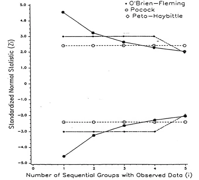
With the interim looks, instead of one single test and one testing procedure with a rejection region, we have many tests to perform at each interim look and the rejections boundaries like on the graph below:
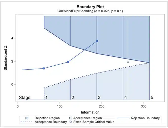
The upper boundary is the efficacy boundary. The dotted low boundary is the futility one. Once the test statistics (blue line with dots) for the single interim look crosses a boundary, you conclude about the efficacy or futility. The image above shows a conclusion to stop the test due to efficacy in the third interim analysis.
A note from our resident statistical expert:
The calculation of such boundaries is based on “alpha-spending” function, and it is pretty complicated even for the advanced statistical experts. As the name suggests alpha spending functions establish α-values spent at each interim analysis given the overall α.
Statisticians use statistical software in order to derive them.
There are different alpha-spending functions named by the names of their inventors:
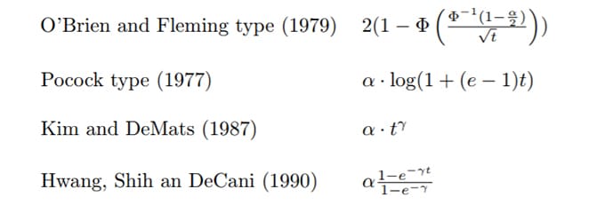
The results can be different depending on the chosen function type.
The graph above is taken from the initial paper of Lan Lan and DeMets (1983) who introduced alpha spending functions. They called this method group sequential design and the sequential groups are just interim look samples.
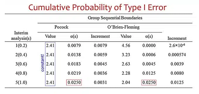
The O’Brien-Fleming alpha spending function has the largest power and is the most conservative in terms that at the same sample size, the null hypothesis is the least likely to be rejected at an early stage of the study.
The table below illustrates the thresholds for the test statistics for the O’Brien-Fleming and Pocock functions. The Pocock thresholds are constant along the time. You can observe how the type I error cumulates until reaching the value of 0.025 for the last interim look. This is the idea of keeping a type I error not inflated by the multiple interim looks.
Can I stop if I see that variations are performing much worse than the control but I am at half the sample size?
Wait for the interim look and then make a test to decide whether you can stop. And if the interim look is not planned you must wait until the end of the study OR recalculate the sample size for the new data. That is somehow another approach for the adaptive design.
Bayesian approach for early stopping
There is also a Bayesian approach to the problem. Zhu and Yu [2] proposed a method that, based on simulations provides larger power than the corresponding frequentist sequential design. “ It also has larger power than traditional Bayesian sequential design which sets equal critical values for all interim analyses.” They show that adding a step of stop for futility in the Bayesian sequential design can reduce the overall type I error and reduce the actual sample sizes.
What is the formula for calculating A/B test sample size: Examples of A/B test sample size formulas
Warning! A lot of math ahead. This section is written to demonstrate the math behind calculating sample size. I can only recommend reading it for our blog readers who are really interested in math!
Here I will present the mathematical formulas for calculating the sample size in an AB test. This is the method implemented in most available online calculators comparing the two conversion rates.
[latex]{ n }_{ 1 }=[/latex][latex]\frac { \bar { \varrho } }{ \left( { \varrho }_{ 1 }-{ \varrho }_{ 2 } \right) 2 }[/latex][latex]\left( { z }_{ \beta }+{ z }_{ \alpha /2 } \right) 2[/latex]
Where:
[latex]{ \varrho}_{ 1 }[/latex])and([latex]{ \varrho}_{ 2 }[/latex] are the true conversion rates
[latex]\bar { \varrho }[/latex] is the pooled variance estimator
α is significance level (Typically α=0.05)
β is desired power (Typically β=0.8)
[latex]{ z }_{ \beta }[/latex] and [latex]{ z }_{ \alpha /2 }[/latex] are critical values for given parameters α and β
Typically for α=0.05 [latex]{ z }_{ \alpha /2 }[/latex] equals 1.96 and for β=0.8 is equal [latex]{ z }_{ \beta }[/latex] 0.84.
We use here pooled estimator for variance assuming that variances (variability) for both conversion rates are equal.
Therefore we have:
[latex] \bar { \varrho} ={ \bar { { \varrho}_{ 1 } } }\left( 1-\bar { { \varrho}_{ 1 } } \right) +\bar { { \varrho}_{ 2 } } \left( 1-\bar { { \varrho}_{ 2 } } \right) [/latex]
Note that [latex]\bar { { \varrho }_{ 1 } }[/latex] is the estimator of the true [latex]{ \varrho }_{ 1 }[/latex]. Hence [latex]\bar { { \varrho }_{ 1 } } ={ r }_{ 1 }[/latex] , where [latex]{ r }_{ 1 }[/latex]is the conversion rate for the control observed in a sample.
If we do not assume equal variances for both conversion rates then the formula is slightly different.
Example calculation of equal-sized groups
Let’s assume that we would like to compute the minimal sample size to detect a 20% increase in conversion rates where the control conversion rate is 50%.
Let’s plug in the numbers into the formula.
The control conversion rate [latex]{ \varrho}_{ 1 }[/latex] is equal 50%
The variation conversion [latex]{ \varrho}_{ 2 }[/latex] is equal to 60%.
We assume an equal ratio of visitors to both control and variation.
We will use a power we assume standard minimal 0.8.
We assume a significance level of 0.05.
First, we calculate the pooled variance estimator.
[latex]\bar { \varrho }[/latex] =0.5(1 – 0.5) + 0.6(1 – 0.6)=0.25 + 0.24=0.49
For α=0.05 [latex]{ z }_{ \alpha /2 }[/latex] equals 1.96 and for β=0.8 [latex]{ z }_{ \beta }[/latex] equals 0.84. Therefore we have:
[latex]n=\frac { 0.49 }{ 0.01 }[/latex] [latex]{ \left( 1.96+0.8 \right) }^{ 2 }=98\cdot 7.84\quad =\quad 384.16[/latex]
Hence the minimal sample size is 385 in each group (control and variation).
Unequal sized groups
The method described above assumes the AB test will run in two equal sized groups. So, the control receives 50% and the variation receives 50%. However, this may not always be the case in practice. If you are introducing a new design, you might drive more visitors to the control first before pushing more visitors at a later stage to the variation.
In this case, the first step is to calculate the total sample size assuming that the groups are equal sized. Then this total sample size N can then be adjusted according to the actual ratio of the two groups (k) with the revised total sample size (N‘) equal to the following:
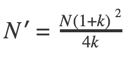
and the individual sample sizes in each of the two groups are N‘/(1 + k) and kN‘/(1 + k).
I attempted to add the interim looks to this example but in all honesty, I just could not do them manually. I asked our resident statistics genius to help me, and her reply was,” The formula to derive the thresholds based on alpha spending function is way too complicated and readers will not appreciate it!”
Sample size calculation using a confidence interval (CI)
Another way to calculate the sample size for an AB test is by using the confidence interval. From the definition, the confidence interval is a type of interval estimate that contains the true values of our parameter of interest with a given probability.
For example, if 95% CI for a single conversion rate is equal [0.2,0.8], that means that the true values of this conversion rate are within this interval. In other words, if we could repeat our experiment many times, the observed conversion rates would fall in this interval in 95 per 100 experiments.
The confidence interval is always symmetric around the computed sample estimate. So for the [0.2,0.8], the single estimate is 0.5. It is the middle of the interval. The length of the interval is therefore 0.6.
For the comparing two conversion rates, we usually do not estimate two intervals for each rate but one interval for the difference between the two conversion rates.
The sample size can be calculated based on the desired length for this interval.
The formula for the 95%CI (LL, UL) is the following:
LL= [latex]\bar { { \varrho }_{ 1 } } -\bar { { \varrho }_{ 2 } } -[/latex] [latex]{ z }_{ 1-\alpha /2 }\sqrt { \frac { \bar { { \varrho }_{ 1 } } \left( 1-\bar { { \varrho }_{ 1 } } \right) }{ { n }_{ 1 } } +\frac { \bar { { \varrho }_{ 2 } } \left( 1-\bar { { \varrho }_{ 2 } } \right) }{ { n }_{ 2 } } } [/latex]
UL=[latex]\bar { { \varrho }_{ 1 } } -\bar { { \varrho }_{ 2 } } +[/latex][latex]{ z }_{ 1-\alpha /2 }\sqrt { \frac { \bar { { \varrho }_{ 1 } } \left( 1-\bar { { \varrho }_{ 1 } } \right) }{ { n }_{ 1 } } +\frac { \bar { { \varrho }_{ 2 } } \left( 1-\bar { { \varrho }_{ 2 } } \right) }{ { n }_{ 2 } } }[/latex]
With LL and UP denoting lower and upper limit of the interval.
If 0 falls to the interval the difference between the two rates is not significant.
Having the half of the confidence level with fixed we can calculate the needed sample size:
[latex]n=\frac { { z }^{ 2 }\varrho }{ { d }^{ 2 } }[/latex] , where [latex]z={ z }_{ 1-\alpha /2 }[/latex]
The estimate of the pooled variance [latex]\bar { { \varrho } }[/latex] can be taken from the previous study. In general, it is:
[latex]\bar { { \varrho } } =\bar { { \varrho }_{ 1 } } \left( 1-\bar { { \varrho }_{ 1 } } \right) +\bar { { \varrho }_{ 2 } } \left( 1-\bar { { \varrho }_{ 2 } } \right)[/latex] like we had before.
The width of the confidence interval is a measure of the quality of the rate difference estimation. The more narrow the confidence (less d) the more exact the estimation is.
What is the sample size for the Bayesian A/B test?
There are other methods for calculating the sample size such as the “fully Bayesian” approach and “mixed likelihood (frequentists)-Bayesian” methods.
Both methods are assumed to have Beta prior distributions in each population. In a fully Bayesian approach, the sample is calculated using the desired average length of the posterior credible interval (analog for confidence interval) for the difference between the two conversion rates. In mixed approaches, the prior information is used to derive the predictive distribution of the data, but the likelihood function is used for final inferences.
In the “Bayesian sequential design using alpha spending function to control type I error.”, Han Zhu, Qingzhao Yu state:
“This approach is intended to satisfy investigators who recognize that prior information is important for planning purposes but prefer to base final inferences only on the data”.
The problem with trying to calculate sample size

To run an AB test and get results you can trust and learn from, the population you’re sampling needs to, in theory, be representative of the entire audience you’re trying to target — which is of course an abstract and impossible task.
The thing is, you can’t truly ever tap into every single member of your audience and that’s because it grows and evolves.
The only way out of this is to capture a broad spectrum of your audience to get a reasonably accurate picture of how most of your users are likely to behave.
So, the bigger the sample from your audience, the easier it is to identify patterns that smooth out individual discrepancies from the section of your audience not captured.
Sample size calculator terminology
Baseline conversion rate:
The conversion rate for your control or original version. (Usually labeled “version A” when setting up an A/B test).
You should be able to find this conversion rate within your analytics platform.
If you don’t have or don’t know the baseline conversion rate, make your best-educated guess.
Minimum Detectable Effect (MDE):
The MDE sounds complicated, but it’s actually quite simple if you break the concept down into each of the three terms:
- Minimum = smallest
- Effect = conversion difference between the control and treatment
- Detectable = want you want to see from running the experiment
Therefore, the minimum detectable effect is the smallest conversion lift you’re hoping to achieve.
Unfortunately, there’s no magic number for your MDE. Again, it depends.
As a general rule of thumb, an MDE of 5% is reasonable. If you don’t have the power to detect an MDE of 5%, the test results aren’t trustworthy. The larger the organization and traffic, the more sample the MDE will likely be.
In, and in that tune, the smaller the effect, the bigger your sample size needed.
An MDE can be expressed as an absolute or relative amount.
Absolute:
The actual raw number difference between the conversion rates of the control and variant.
For example, if the baseline conversion rate is 0.77% and you’re expecting the variant to achieve a MDE of ±1%, the absolute difference is 0.23% (Variant: 1% – Control: 0.77% = 0.23%) OR 1.77% (Variant 1% + Control 0.7&% = 1.77%).
Relative:
The percentage difference between the baseline conversion rate and the MDE of the variant.
For example, if the baseline conversion rate is 0.77% and you’re expecting the variant to achieve a MDE of ±1%, the relative difference between the percentages is 29.87% (increase from Control: 0.77% to Variant: 1% = 29.87% gain) or -23% (decrease from Control: 0.77% to Variant 1% =-23%).
In general, clients are used to seeing a relative percentage lift, so it’s typically best way to use a relative percentage calculation and report results this way.
Statistical power 1−β:
Very simply stated, the probability of finding an “effect,” or difference between the performance of the control and variant(s), assuming there is one.
A power of 0.80 is considered standard best practice. So, you can leave it as the default range on this calculator.
A power of 0.80 means there’s an 80% chance that, if there is an effect, you’ll accurately detect it without error. Meaning there’s only a 20% chance you’d miss properly detecting the effect. A risk worth taking.
In testing, your aim is to ensure you have enough power to meaningfully detect a difference in conversion rates. Therefore, a higher power is always better. But the trade-off is, it requires a larger sample size.
In tune, the larger your sample size, the higher your power which is part of why a large sample size is required for accurate A/B testing.
Significance Level α:
As a very basic definition, significance level alpha is the false positive rate, or the percentage of time a conversion difference will be detected — even though one doesn’t actually exist.
As an A/B testing best practice, your significance level should be 5% or lower.
This number means there’s less than a 5% chance you find a difference between the control and variant — when no difference actually exists.
As such, you’re 95% confident results are accurate, reliable, and repeatable.
It’s important to note that results can never actually achieve 100% statistical significance.
Instead, you can only ever be 99.9% confident that a measurable conversion rate difference can truly be detected between the control and variant.
Additional Resources
1. What to do when your AB tests keep losing
2. What they don’t tell you about A/B testing velocity
4. What are the features of a good A/B testing tool?
5. How to analyze A/B test results and statistical significance in A/B testing
References:
- Lan G., de Mets D.L. Interim Analysis: The alpha spending function approach. (1994) SM, Vol 13, 1341-1352.
- Per Broberg. Sample size re-assessment leading to a raised sample size does not inflate type I error rate under mild conditions. 2013. PMC.
- Zhu H., Yu Q.A Bayesian sequential design using alpha spending function to control type I error. 2017 SMMR.