Are you tired of running A/B tests and ending up with inconclusive results? There’s another dilemma about which test method to choose and which fits your goals the best.
Many marketers and product managers face these challenges when optimizing their websites or products. But don’t worry, there’s a solution to your pain points: understanding the Frequentist and Bayesian approaches to A/B testing.
In this article, we’ll talk about these two most prominent A/B testing methods. We’ll explore their methodologies, advantages, disadvantages, and when to use each. By the end, you’ll have a clearer understanding of which method is better suited for your testing needs, helping you make more informed decisions and achieve more reliable results.
Frequentist Approach
The Frequentist approach is a traditional way of looking at statistics based on how often things happen in repeated experiments. It relies on the long-term behavior of data, assuming that probabilities are related to the frequencies of events in repeated trials.
In the context of A/B testing, the Frequentist approach compares two versions (A and B) by looking at the observed differences in outcomes – click-through rates, conversion rates, or any other key performance indicators.
Imagine you’re flipping a coin. If you flip it 100 times and it comes up heads 55 times, you might say, “This coin seems fair because heads came up about half the time.”
Let’s say you’re testing two website designs, A and B, to see which one gets more clicks. You show design A to 100 people and design B to another 100 people. If design A gets 60 clicks and design B gets 40 clicks, you might think, “Design A is probably better.”
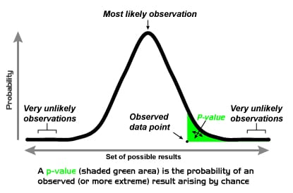
But you want to be sure it’s not just by chance. So, you use the Frequentist approach to calculate the likelihood that the difference in clicks is real, not just luck. If this likelihood (called the p-value) is very low, you can confidently say that design A is better.
The Frequentist approach is a careful way of making decisions based on how often things happen in tests or experiments. It helps you determine if what you see is likely true or just a fluke.
Methodology in A/B testing: Null Hypothesis and Alternative Hypothesis
Step 1. In Frequentist A/B testing, the process begins with formulating two hypotheses.
- Null Hypothesis (H0): This hypothesis assumes that there is no significant difference between the two versions being tested. This is the assumption that there’s no difference or effect. For example, if you’re testing two website designs, your null hypothesis might be “Design A and Design B have the same click-through rate.” Remember, H0 is the default assumption we aim to disprove.
- Alternative Hypothesis (H1): Suggests that there is a significant difference between the two versions. This is what you’re trying to prove. For example, “Design A has a higher click-through rate than Design B.”
So, how does this translate to A/B testing?
The goal of the A/B test is to determine whether there is enough evidence to reject the null hypothesis in favor of the alternative hypothesis.
Imagine testing two website layouts. H0 would be “both layouts convert equally.” We collect data on conversions (potion successes!), calculate p-values, and voila! Based on the p-value, we declare a winner or remain undecided.
Before formulating your two hypotheses, don’t forget to define your objective and metrics.
What do you want to test? Are you optimizing conversion rates, engagement, or something else? Clearly define the primary and secondary metrics you’ll use to measure success.
Step 2. The next step is to choose your variations and sample size:
- Variation Variety: Define the variations you want to test. This could include different versions of a product page headline, call-to-action buttons, or entire website layouts. Ensure the variations are distinct enough to yield meaningful results.
- Sample Size: Use a power analysis tool to determine the minimum sample size needed for statistically significant results. This depends on the expected effect size, desired significance level, and power. Remember, a larger sample size increases the likelihood of detecting true differences but also requires more data collection time.
Step 3. Next, decide on the significance levels and p-values.
- Deciding on a Significance Level: This pre-defined threshold determines the confidence level required to reject H0. It helps decide when to say there’s a real difference between the two versions. Commonly used values are 0.05 (95% confidence) or 0.01 (99% confidence).
Choosing a lower alpha makes you more cautious, requiring stronger evidence for a significant difference, while a higher alpha increases the risk of false positives (mistaking chance for a real effect). - Looking at the p-Value: p-value is a crucial concept in Frequentist A/B testing and acts as your evidence meter. It represents the probability of observing your test results if H0 (no difference) were true. Think of it as the chance of seeing such a difference purely by random chance. If this number is smaller than your significance level, you can say there’s a real difference.
- P-value and alpha: The significance level (alpha) sets the bar for how low the p-value needs to be for you to reject H0. For example, with alpha = 0.05, if your p-value is less than 0.05 (5%), you have strong evidence against H0 and can declare a statistically significant difference.
Step 4. Finally, design and implement the test:
- Randomized Royalty: Ensure your test is truly randomized. Users should be randomly assigned to each variation, eliminating bias and ensuring fair comparison. Ensure you take assistance from online A/B testing tools like FigPii and Optimizely to simplify the process.
- Distribution Detective: Monitor user distribution across variations throughout the test. Watch for imbalances that might skew results and take corrective measures if needed. For example, similar traffic volumes for each variation should be ensured to avoid biased data.
- Data Quality Duchess: Be vigilant about experiment data quality. Regularly monitor for errors, missing values, or suspicious patterns that might compromise your conclusions. Clean and reliable data is the cornerstone of robust analysis.
Quick Tips for Doing It Right
- Keep Things Fair: Ensure other factors don’t affect your test results. Randomly assigning people to different versions can help.
- Check Your Results Carefully: Keep an eye on your p-value, but don’t check too often, as it can mess up your results.
- Think About What It All Means: Even if you find a significant difference, make sure it’s meaningful for your goals.
Advantages and Disadvantages of Frequentist A/B Testing Method
The Frequentist approach – emphasizing hypothesis testing and p-values – is a cornerstone of A/B testing. But it comes with its own set of advantages and disadvantages.
Advantages of the Frequentist Approach:
- Easy to understand and interpret: The Frequentist approach is based on well-established statistical principles, making it relatively accessible even if you have a basic understanding of statistics. The concept of p-values and significance levels is also pretty straightforward, making it easier to communicate results.
- Controls for false positives: By pre-defining the significance level (alpha), the Frequentist approach inherently reduces the risk of declaring a significant difference when it’s just due to chance. This helps maintain scientific rigor and avoids misleading conclusions.
- Well-documented and supported: The Frequentist approach boasts a long history in various scientific fields, leading to extensive documentation and abundant resources. This knowledge base facilitates learning and ensures you leverage a well-tested methodology.
- Widely used and accepted: The Frequentist approach remains popular in A/B testing across diverse industries due to its simplicity and clarity. Its widespread adoption allows for easier comparison of results from different studies and facilitates collaboration within the A/B testing community.
Disadvantages of the Frequentist Approach:
- Limited to point estimates: The Frequentist approach primarily provides point estimates, like the observed difference between variations. It doesn’t offer direct insights into the probability or range of possible values for the true effect size.
- Reliance on large sample sizes: To achieve statistically significant results, the Frequentist approach often requires larger sample sizes than other methods like the Bayesian approach. This can be time-consuming and resource-intensive, especially for smaller businesses or startups.
- Sensitivity to prior knowledge: The Frequentist approach doesn’t readily consider prior knowledge or expectations about the potential effect size. This can lead to missed opportunities or inaccurate conclusions, especially when dealing with limited data.
- Potential for p-hacking: Focusing on p-values can incentivize practices like “p-hacking,” where researchers manipulate data or analysis methods to achieve a desired p-value.
Bayesian Approach
The Bayesian method in A/B testing is a statistical framework that incorporates prior knowledge or beliefs (like the detective’s intuition) alongside data from the experiment to estimate the true effect size.
It uses Bayes’ theorem, a powerful equation, to update its understanding of the variations’ being tested as data accumulates.
Unlike the Frequentist approach, which relies solely on data from the current experiment, the Bayesian approach allows for updating probabilities as new data becomes available.
Let’s consider it with an example.
Imagine you’re trying to guess how likely your friend will win a game. Before the game starts, you have an initial guess based on what you know about your friend’s skills. This is your “prior” belief.
You watch your friend play and gather new information as the game progresses. In the Bayesian approach, you use this new information to update your initial guess. This updated guess is called the “posterior” probability.
The beauty of the Bayesian approach is that it’s a continuous process. As more and more data comes in, you keep updating your beliefs. It’s like constantly adjusting your guess based on the latest evidence.
Let’s say you want to predict whether it will rain tomorrow.
Your prior belief might be based on the fact that it’s been raining a lot recently, so you think there’s a 70% chance of rain.
Now, suppose a weather forecast predicts sunny weather. You combine this new information with your prior belief to update your prediction. After considering the forecast, you might adjust your belief to a 40% chance of rain. This new probability is your posterior belief.
E-commerce platforms can also leverage the Bayesian approach to personalize product recommendations, dynamically tailoring them to each user’s browsing history and purchase behavior.
The Bayesian approach is a way of doing statistics that combines what you already know with new data to make better predictions. It’s like continuously refining your guesses as you learn more information.
Methodology in A/B testing:
Here’s how to go about it:
Step 1: Define your objective and metrics:
- What are you aiming to test? Like the Frequentist approach, clearly define your objective and identify the key performance indicators (KPIs) to measure success.
Step 2: Define your “Prior”:
- Prior Distribution: Instead of H0 and H1, like in the Frequentist approach, you’ll define a prior distribution for your expected effect size. Start with a prior belief about the metric you’re testing (e.g., conversion rate).
This belief is based on past data or expert opinion. For example, if, based on past tests, you expect Layout A to convert 2% better than Layout B, your prior distribution might be centered around a 2% difference with some uncertainty.
Step 3: Choose your variations and sample size:
- Like the Frequentist approach, select the variations you want to test and determine the minimum sample size needed for reliable results. Consider factors like expected effect size, desired precision, and prior knowledge when choosing the sample size.
Step 4: Update your belief:
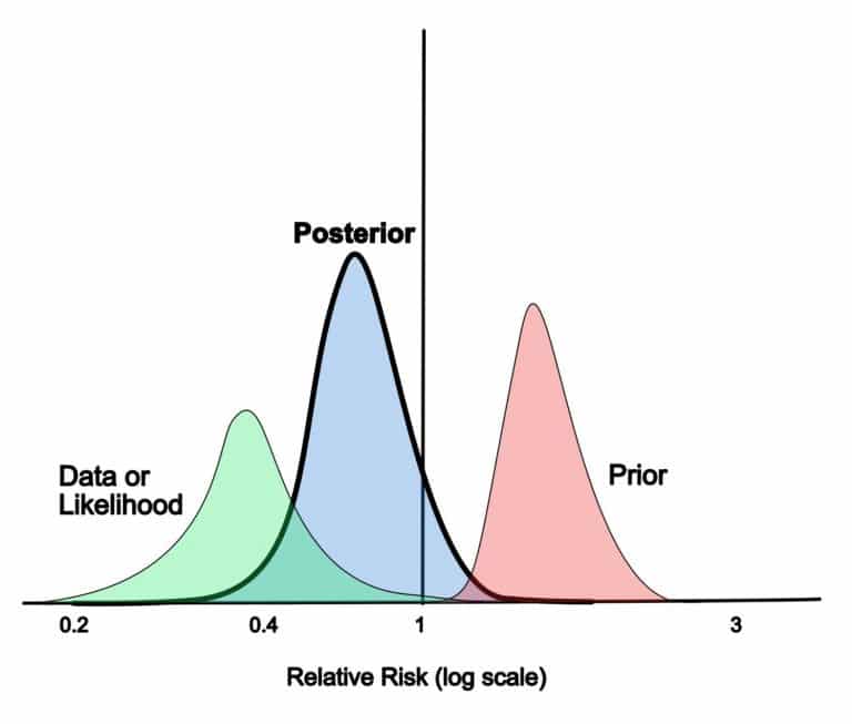
- Posterior Distribution: Use the data from your A/B test to update your prior belief. This is done using Bayes’ theorem, which combines your prior with the likelihood of observing the data. The result is the posterior distribution, representing your updated belief about the conversion rates.
Step 5: Make decisions
- Analyze results and draw conclusions: Instead of p-values, the Bayesian approach provides posterior distributions for the effect size. This shows the range of possible values and their associated probabilities. Analyze these distributions and their credibility intervals to draw conclusions about the true difference.
- Final decision-making: Based on the posterior distributions and your understanding of the context, make informed decisions about which variation to adopt or whether further testing is needed. Remember, Bayesian conclusions are based on data and prior knowledge, not just a single p-value.
Step 6: Continuous learning
- Updating with new data: As more data becomes available, you can update your posterior distribution again. This helps you continuously learn and refine your beliefs.
In simple terms, the Bayesian approach in A/B testing is like making a smart guess, checking it with real data, and then updating your guess to make better decisions. And the more you learn, the smarter your decisions can be!
Quick Tips for Doing It Right
Here are three major tips for doing Bayesian A/B testing right:
- Choose an Appropriate Prior: Start with a prior that reflects your existing knowledge or beliefs about the metric you’re testing. This sets a solid foundation for your analysis.
- Interpret Probabilities Carefully: Focus on the probability that one version is better than the other rather than just looking at average results. This gives you a more nuanced understanding of your test outcomes.
- Update with New Data: Be prepared to update your analysis as more data comes in continuously. This allows you to refine your conclusions and make more informed decisions over time.
Advantages and Disadvantages of Bayesian A/B Testing Method
Advantages of the Bayesian Approach:
- Leverages prior knowledge: Unlike the Frequentist approach, which starts with a blank slate, the Bayesian approach allows you to incorporate valuable insights from past experiences or industry trends. This is particularly beneficial when dealing with limited data, where past knowledge can be a guiding light.
- Adapts to new information: The Bayesian approach continuously updates its beliefs as new data arrives, reflecting a more dynamic and data-driven perspective than the Frequentist approach’s fixed hypothesis. This adaptability can lead to quicker identification of significant effects or evolving trends.
- Provides richer insights: Beyond point estimates, the Bayesian approach offers probability distributions for the true effect size. This provides a clearer picture of the range of possible outcomes and associated uncertainties, enabling more nuanced decision-making.
- Flexibility in stopping rules: Unlike the Frequentist approach’s reliance on pre-defined significance levels, the Bayesian approach allows for more flexible stopping rules based on the accumulated evidence and desired level of certainty. This can save time and resources by stopping inconclusive tests early.
Disadvantages of the Bayesian Methodology:
- Subjectivity in prior selection: Choosing the right prior distribution is crucial, as it can significantly influence the results. Biasing the prior can lead to misleading conclusions, requiring careful consideration and justification.
- Computationally intensive: The Bayesian approach often involves complex calculations, which can be computationally demanding, especially for large datasets. This can be a barrier for smaller businesses or individuals with limited computing resources.
- Potential for overfitting: If the prior belief is too strong relative to the data, the Bayesian approach might overfit the results to the prior, leading to inaccurate conclusions. This highlights the importance of carefully selecting and justifying the prior distribution.
- Understanding interpretation: While the flexibility of Bayesian results is valuable, interpreting probability distributions and credibility intervals requires a deeper understanding of statistical analysis and concepts than simply relying on p-values in Frequentist statistics.
Comparison and Considerations: When Should We Use Frequentist vs. Bayesian?
The key differences between Bayesian and frequentist approaches lie in their treatment of prior knowledge, observed data, interpretation of results, and handling of sample size and multiple variations. The choice between the two approaches depends on the following factors:
A. Prior knowledge incorporation:
Bayesian Approach: Bayesian methods allow for incorporating prior knowledge or beliefs about the parameters being tested. This prior information is combined with the observed data to update the beliefs and produce a posterior distribution.
Frequentist Approach: Frequentist methods typically do not incorporate prior knowledge explicitly. They rely solely on the observed data and make inferences based on the likelihood of observing it under different test hypotheses.
B. Treatment of observed data:
Bayesian Approach: In Bayesian statistics, the observed data are used to update the prior beliefs and produce a posterior distribution. This distribution represents the updated knowledge about the parameters being tested.
Frequentist Approach: Frequentist methods treat the observed data as fixed and use them to calculate statistics such as p-values, confidence intervals, and test statistics. The interpretation is based on the probability of observing the data given a specific hypothesis.
C. Interpretation of results:
Bayesian Approach: Bayesian methods provide a probability distribution over the parameters of interest, allowing for direct probabilistic statements about the parameters. This can lead to more intuitive interpretations of results.
Frequentist Approach: Frequentist methods typically provide point estimates, confidence intervals, or hypothesis test results. Interpretations are based on the long-run properties of these estimators or tests, which may not always be intuitive.
D. Handling of sample size and multiple variations:
Bayesian Approach: By incorporating prior information, bayesian methods can handle small sample sizes more effectively. They can also adapt to situations with multiple variations by adjusting the prior distributions accordingly.
Frequentist Approach: Frequentist methods often require larger sample sizes to achieve desired levels of statistical power. Handling multiple variations may involve adjustments to significance levels or the use of multiple testing corrections.
Common Use Cases of the Frequentist and Bayesian Approach
Frequentist Approach Use Cases:
- Large-scale A/B tests where sample size is not an issue.
- Regulatory environments where a binary decision is required.
- Situations where the goal is to determine if an effect exists.
Bayesian Approach Use Cases:
- Early-stage product development with small sample sizes.
- Tests where incorporating expert knowledge is valuable.
- Continuous testing environments where decisions need to be updated frequently.
Bayesian vs. Frequentist: Finding the Right Fit for Your A/B Testing
When finding an A/B testing method, there’s no one-size-fits-all winner. Each method has strengths and weaknesses; the best choice depends on your specific testing needs.
For example, the Frequentist approach might be your go-to if you have a large sample size and need clear, binary decisions. It’s straightforward and widely accepted, making it a reliable choice for many standard A/B tests.
On the other hand, if you’re working with smaller sample sizes or want to incorporate prior knowledge into your testing, the Bayesian approach could be your best bet. It’s flexible and provides richer insights, allowing you to update your results based on updated data.