I have meant to write this post for a long time. There has been a lot written about one-tailed vs. two-tailed tests. However, most of the articles approach the topic from a purely statistical perspective providing many formulas but do not show how to do the calculations. Others articles approach the issue from a high-level business perspective. So, here is my attempt to delve deep into the topic. Some sections in this article are heavy on stats and formulas. If you are not interested in these, you can skip them! Special thanks to our data sciences team that checked and rechecked the math on the article.
Most A/B testing platforms do not provide the option to choose between one-tailed vs. two-tailed analysis. Moreover, until 2015, several popular testing platforms relied on one-tailed in statistical analysis.
The same applies to many other disciplines where having to choose between a one-tailed vs. two-tailed is rarely encountered since the majority of statistical software only offers two-tailed analysis as the single option.
There is a common belief that two-tailed tests are generally “better” in some way, leading to more accurate and more reliable results.
This is an apparent misconception.
Surprisingly, these misconceptions originate from wrong guidelines present in many statistical publications. Let’s take a look at the following from Wikipedia:
“A two-tailed test is appropriate if the estimated value may be more than or less than the reference value, for example, whether a test taker may score above or below the historical average. A one-tailed test is appropriate if the estimated value may depart from the reference value in only one direction, for example, whether a machine produces more than one-percent defective products.”
This sentence is misleading since one is often interested in discovering one direction difference (did the test generate an uplift) even when both directions are possible.
When conducting an AB test, we are typically interested in finding out if a variation generated a generated a statistically significant increase in conversions. Thus, for these cases, a one-sided test is appropriate since we would like to find a difference in one particular direction. According to Kylie Vallee:
“If you’re running a test and only using a one-tailed test, you will only see significance if your new variant outperforms the default. There are 2 outcomes: the new variants win or we cannot distinguish it from the default.”
A two-tailed test should be used when we would like to discover a statistically significant difference in any direction. In this case, we examine if the variation generated a statistically significant increase or a decrease in conversions.
This article covers several issues around the choice between one-tailed vs. two-tailed tests that you should be aware of if you are conducting AB testing.
However, the decision on which approach to choose should always be based on the aim of the experiment and the question of interest, not the technical differences between the two tests. These technical differences are merely a consequence of their statistical construction.
Let’s start with the real-life examples.
Example 1: Using statistical methods with an e-commerce store
Let’s say an e-commerce store is looking to modify product pages to increase the website conversions rate.
The conversion rate for the product page, in that case, is defined as the number of orders divided by the number of visitors to product pages. The marketing team is considering three new designs for the product page. Their aim is to choose the best design out of the four available ones: the existing design and three new ones.
We will show below how to use statistical methods to make such a decision, using the conversion rate as a criterion.
Example 2 – Statistical methods with a SaaS website
A SaaS website is looking to increase its number of subscribers by modifying its pricing page.
The conversion rate for the pricing page is defined as the number of subscriptions divided by the number of visitors to the pricing page.
The marketing team is considering three new designs for the pricing page. The team would like to decide if any of the new designs are better than the existing one, i. e. it leads to more subscribers.
Also, in this case, statistical methods allow for making such a decision using the conversion rate as a criterion of comparison.
Step 1: Formulating One Tailed /Two Tailed Hypothesis

To address these examples through A/B testing, we will first formulate your hypothesis of interest.
For both examples, the hypothesis is that the conversion rate for one of the three new page designs ([latex]\rho _{N}[/latex]) is equal to the conversion rate for the current design ([latex]\rho _{C}[/latex]). This called a null hypothesis and is denoted by H0. Therefore:
H0: [latex]\rho _{N}=\rho _{C}[/latex]
Then you formulate your alternative hypothesis H1. The alternative hypothesis can be one of the three possible forms:
H1:[latex]\rho _{N}[/latex] not equal [latex]\rho _{C}[/latex] (less or greater)
or
H1: [latex]\rho _{N}[/latex] greater than[latex]\rho _{C}[/latex] (right-sided) – one of the variations will cause an uplift in conversions
or
H1:[latex]\rho _{N}[/latex] less than [latex]\rho _{C}[/latex] (left-sided) – one of the variations will cause a drop in conversions
In the first case, you do not assume that the new design will generate an increase or decrease in conversions. The first type of test is called a two-tailed test.
In the last two cases, you assume the impact of the new design. This is referred to as a one-sided test (left-or right-sided)
In a pure statistical world, you would typically conduct three different AB tests since you have three variations. Each test will run the original against one of the variations. Also, for each test, we will use the same procedure of hypothesis formulation. It is also essential to decide IN ADVANCE what form of the alternative hypothesis you would like to test.
In other words, this choice should NOT be a data-driven but a consequence of a question of interest. You will ask yourself:
- Do you care to see if a variation generates a significant change, or
- Do you care to see if a variation generates a significant uplift, or
- Do you care to see if a variation generates a significant drop
Your decision to use a one-tailed test to prove a statistically significant difference in a particular direction, but not in the other direction.
Typically, you would run a single AB test with three variations against the control. However, you should be aware that doing so could cause a “multiple testing” problem which is a common problem in statistics. It reflects the increasing the probability of discovering false positive significant result as more variations are introduced to a test. There are several solutions to this problem which I will discuss in a later article ( correction for multiple testing or using other statistical methods).
Step 2: Conducting the A/B Test
After formulating your hypothesis, you are ready to conduct the AB test. As the testing software collects data on each of the variations, it starts to do some computational work to determine the performance of the control and the different variations.
The A/B testing software computes the z-score (test statistics) which is a mathematical formula based on the observed values of conversion rates for the variations ([latex]r_{N}[/latex]), the conversion rate for the control ([latex]r_{C}[/latex]), the number of visitors to the variation ([latex]n_{N}[/latex]) and the number of visitors to the control([latex]n_{C}[/latex]).
If we assume the same (true) variances for both rates, the Z-score has the form:
[latex]Z=\frac{r_{N}-r_{C}}{\sqrt{r(1-r)(\frac{1}{n_{N}}+\frac{1}{n_{C}})}}[/latex]
r is a pooled proportion (conversion rate) calculated as:
[latex]r=\frac{r_{N}+r_{C}}{n_{N}+n_{C}}[/latex]
In a more general case, when the variances for the two rates are different we cannot use the pooled r estimator and the Z score is calculated using the following formula:
[latex]Z=\frac{r_{N}-r_{C}}{\sqrt{(\frac{r_{N}(1-r_{N})}{n_{N_{}}}+\frac{r_{C}(1-r_{C})}{n_{C}})}}[/latex]
Notice the difference!
When we created our test hypothesis, we talked about [latex]\rho _{N}[/latex] and [latex]\rho _{C}[/latex]. When we conducted the test, we are using [latex]r_{C}[/latex] and [latex]r_{N}[/latex]
[latex]\rho _{N}[/latex] and [latex]\rho _{C}[/latex] are hypothetical conversion rates for the whole populations of users. They are the assumed conversion rates for all visitors who will come to the page.
[latex]r_{C}[/latex] and [latex]r_{N}[/latex] are the actual observed conversion rates while are conducting the AB test which runs for a sample from the population.
Why is this important?
This is the biggest challenge of AB testing! You run the test for a specific period and observe the conversion rates for the control and the variations. You are collecting the behavior of a sample of your users and using that sample to judge how the whole population will react to these designs.

Here is a highly sanitized example to drive this point home:
Let’s say that you have a page that gets 10,000 visitors/day. You run an AB test for a period of 14 days. So during that period, your page gets 140,000 visitors. Before launching the test, your boss tells you that you will use the winning design from the AB test for the next 365 days. In this case, the population is 10,000 * 365 = 3,650,000 visitors.
When you conclude the AB test, you will use the data from the reaction of 140,000 visitors to judge the response of 3,650,000 visitors. So, you are using data from 3.8% sample to judge the performance of the population.
Step 3: Decision Making
Critical region
The critical region is a set of outcomes of a statistical test for which the null hypothesis is to be rejected.
Statistical testing using critical region -step by step:
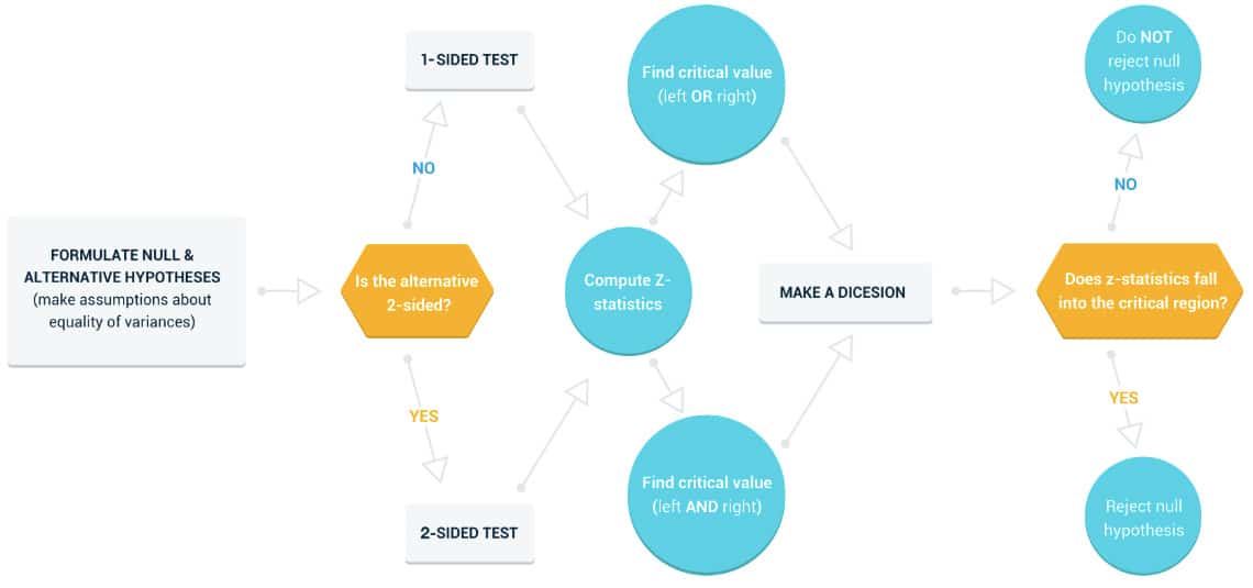
Critical region in two-tailed A/B tests
Let’s consider a numerical example for the above step-by-step analysis.
Let us assume that we observe two conversion rates:
- The control conversion rate 70% (100 visitors, 70 conversions)
- Variation conversion rate 80% (100 visitors, 80 conversions)
For the sake of simplicity, I used a small number of visitors and conversions. I also assumed that both the control and the variation will get the same number of visitors. I am also assuming equal variances for both rates in the population.
Formulate null and alternative hypotheses
Let’s assume that we want to test if the new design will result in an increase or a drop in conversion so we will use a two-tailed AB test.
Calculate Z score
First we calculate pooled conversion rate:
[latex]r=\frac{80+70}{100+100}=\frac{150}{200}=0.75[/latex]
[latex]Z=\frac{0.8-0.7}{\sqrt{0.75(1-0.75)(\frac{1}{100}+\frac{1}{100})}}[/latex]=
[latex]\frac{0.1}{\sqrt{0.1875\cdot
0.02}}=\frac{0.1}{\sqrt{0.00375}}=\frac{0.1}{0.0612}=1.633[/latex]
Find critical values
After calculating of the z-score, we check if this value fails into so-called critical region.
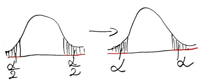
The critical regions are the x-axis part of the shaded areas on the pictures below. They look differently for different types of alternative hypotheses: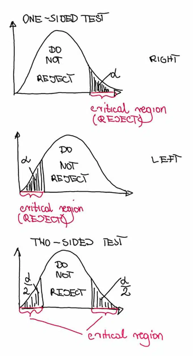
The critical region (red part on the x-axis) is placed on both sides for two-sided test and on one side for the one-sided test.
Since we are interested in conducting the two-sided test, so the critical region looks like on the third picture. It consists of the two intervals : (-∞;-critical value] and [critical value;+∞).
The negative critical value (- critical value) is the point on the x-axis where the red region finishes on the left side and when it begins on the right side. [latex]z_{1-\frac{\alpha }{2}}[/latex]
We take the critical value from the special statistical tables. The critical value is a value determined by the significance level (see the next section) and is denoted for the two-sided test as.
For our example, it will be equal to 1.96. So the critical region in our example has the form:
(-∞;-1.96] and [1.96;+∞)
Make a decision
Since our computed Z score value equals 1.63 it does not fail in the right part of the critical region. Therefore we do not reject the null hypothesis.
Therefore, we cannot state that one of the designs will increase conversion rates more than the other. All we can state is that we do not have enough evidence to conclude the relevant difference between the control and the variation.
The picture shows the distributions of the Z-score. This illustrates all possible values of the statistical test formula that could be obtained if you could repeat your experiment very many times. As can be noticed they are typically distributed (around the zero mean), so the density curves are bell-shaped. They are referred to as normal or Gaussian distribution. It is one of the most popular statistical distributions. According to Cliffs notes website:
“The decision of whether to use a one‐ or a two‐tailed test is important because a test statistic that falls in the region of rejection in a one‐tailed test may not do so in a two‐tailed test, even though both tests use the same probability level.”
Normal distribution widely used since it describes most of the mechanisms in nature. Like any statistical distribution, it illustrates the proportions of some continuous feature in a population. For example, if you measure the age of some defined group like the age of users visiting the website then, based on the mathematical theory, it will have the normal distribution, provided that we have a large sample. Statisticians say that “everything is normal sooner or later.”
The critical thing about this distribution is that is centered around the mean of the observed feature (mean age in the example ), and it can be more or less spread around it depending if the variability in the observed group is less (less spread) or larger (widespread).
Critical region in the one-tailed A/B test
What would be our conclusion if we would like to perform the right-sided test, so testing that the new design will convert more visitors compared to the control? Then the critical region would look like on the first picture.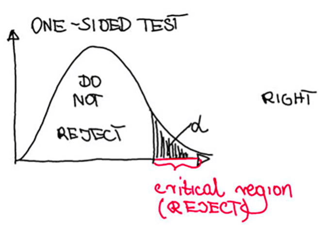
The value of the Z score remains the same.
So it is still 1.63.
Find critical value
The critical value [latex]z_{1-\alpha }[/latex] is now 1.64 so the critical region is of the form [1.64,+∞]
Make a decision
Since the test statistic does not fail in this interval, we cannot reject the null hypothesis about the equality of the two designs. Thus, we cannot conclude that the new design is better than the current one. However, we see that we are now closer to the critical region than before. According to Surbhi S.:
“One-tailed test represents that the estimated test parameter is greater or less than the critical value. When the sample tested falls in the region of rejection, i.e. either left or right side, as the case may be, it leads to the acceptance of alternative hypothesis rather than the null hypothesis.”
The results would be much different if we assume non-equal variances for both groups!
Z score will be then 1.644 (I am skilling the calculations but the formulas are above!).
In this case, the Z-score falls into the critical region for the right-sided test. Therefore, we can conclude that the new design does increase conversion rates.
As you can see the assumptions are crucial here and the right-sided test has more chance to detect the difference.
Do we need to do it the Z-score calculation by hand?
In practice, the AB testing software or statistical software does all the calculations for us.
As a result, it provides so-called p-values as a final result of a test. P-value is the probability of rejecting the null hypothesis when H0 is true. If the P-value is less than the significance level (usually 0.05), than we say the result is significant. If it is greater or equal to the significance level, then we state that the difference is not significant.
Significance level
The significance level of a test (sometimes referred to as Alpha “α”) is the shaded area.
The α false null hypothesis (concluding that the new design is different from the existing one) you make this right decision with the probability of 1-α (see the smiley face in the first row on the graph below).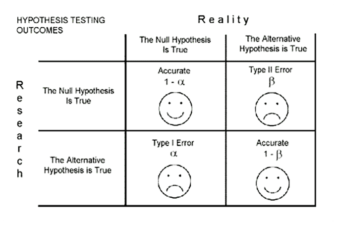
You have to decide how big the significance level α can be for your test. Typically we use 0.05. When you reject the null hypothesis, statisticians say that the test is significant.
The probability that you were able to detect the difference between the control and the variation, if it exists, is called power and is denoted by 1-β. (See the table above).
- If you fail to reject the null hypothesis, you made the right decision if H0 was true.
- if you fail to reject the null hypothesis, you made the wrong decision if H0 was false. This is typically referred to as type II error (β).
In the last case, statisticians say that your study was underpowered meaning that you didn’t have enough evidence to detect the true difference. The smaller the difference between the true rates the more data you need to detect it (more traffic). It is like looking through a small magnifying glass. You need a bigger one if you are looking at a tiny object.
Confidence intervals for one-tailed vs. two-tailed tests
We typically like to construct a “confidence interval” to determine the true difference between the two rates.
A confidence interval is an interval that contains all possible values of that difference that you would obtain if you could repeat your experiment very many times, with the probability.
For example, for 100 repetitions of the same experiment, the computed difference between the rates would fail into 95%CI in 95 cases.
Calculating the confidence interval for the two-tailed test
First, we need to calculate the limits of the interval [LL,UL].
[latex]LL=r_{N}-r_{C}+z_{1-\frac{\alpha
}{2}}\sqrt{\frac{r_{N}(1-r_{N})}{n_{N}}+\frac{r_{C}(1-r_{C})}{n_{C}}}[/latex]
[latex]UL=r_{N}-r_{C}-z_{1-\frac{\alpha
}{2}}\sqrt{\frac{r_{N}(1-r_{N})}{n_{N}}+\frac{r_{C}(1-r_{C})}{n_{C}}}[/latex]
For the two-sided test those limits can be calculated as follows:
[latex]UL=r_{N}-r_{C}+z_{1-\frac{\alpha }{2}}\cdot
\sqrt{\frac{r_{N}(1-r_{N})}{n_{N}}+\frac{r_{C}(1-r_{C})}{n_{C}}}=0.8-0.7+1.96\sqrt{\frac{0.8(1-0.8)}{100}+\frac{0.7(1-0.7)}{100}}=0.1+1.96\sqrt{\frac{0.16}{100}+\frac{0.21}{100}}=0.1+1.96\sqrt{\frac{0.37}{100}}=0.21[/latex]
[latex]LL=r_{N}-r_{C}-z_{1-\frac{\alpha }{2}}\cdot[/latex]
[latex]\sqrt{\frac{r_{N}(1-r_{N})}{n_{N}}+\frac{r_{C}(1-r_{C})}{n_{C}}}=0.8-0.7-1.96\sqrt{\frac{0.8(1-0.8)}{100}+\frac{0.7(1-0.7)}{100}}=0.1-1.96\sqrt{\frac{0.16}{100}+\frac{0.21}{100}}=0.1-1.96\sqrt{\frac{0.37}{100}}=-0.019[/latex]
This is under of assumption of different variances for both rates. In case of a pooled rate estimator the formula under the squared root changes like for the Z test statistics. So for our numerical example from paragraph we obtain:
Therefore the 95% CI for the two-sided test has the form: [-0.019;0.219].
It means that the true values of the difference between the two rates vary from -0.019 to 0.219.
Notice that the interval contains zero, which means that it possible that there is no difference between the means at all. Therefore, we state that the result is not significant.
Calculating the confidence interval for the one-tailed test
We can also compute the confidence interval for a one-sided test.
Confidence interval, in this case, has the form of (-∞;UL] for right-sided test and [LL;+∞) for the left-sided test. For the right-sided test the formula for UL is as follows:
[latex]LL=r_{N}-r_{C}+z_{1-\alpha
}\sqrt{\frac{r_{N}(1-r_{N})}{n_{N}}+\frac{r_{C}(1-r_{C})}{n_{C}}}[/latex]
And for the left-sided test the formula for UL is of the analogical form:
[latex]UL=r_{N}-r_{C}-z_{1-\alpha
}\sqrt{\frac{r_{N}(1-r_{N})}{n_{N}}+\frac{r_{C}(1-r_{C})}{n_{C}}}[/latex]
For the two-sided tests, we also check if zero falls into the interval. This is equivalent to statistical testing.
In practice, you use statistical software to compute the confidence interval. If it has the option of only two-sided interval then take a double of alpha and only half of the interval.
The common misunderstanding of two-sided tests
Some marketers think that they can test if a new design will increase conversions or cause a drop (or vice versa) in a one-sided test. So mathematically, that the H0 in two-sided tests is of the form:
H0: [latex]\rho _{N}>\rho _{C}[/latex]
Vs
H1: [latex]\rho _{N}<\rho _{C}[/latex]
Or
H0: [latex]\rho _{N}<\rho _{C}[/latex]
Vs
H1: [latex]\rho _{N}>\rho _{C}[/latex]
That is not correct. The null hypothesis (H0) ALWAYS has an equality (in two or one-sided tests)!
H0: [latex]\rho _{N}=\rho _{C}[/latex]
Only the alternative hypotheses are with inequality signs in one-sided tests.
So, you do not test if a new design causes an increase vs. causes a drop in conversions in a one-tailed test.
You test if:
the new design conversion rate is equal to the control conversion rate
versus
the new design conversion rate is higher than the control.
Therefore, when you do not reject the null hypothesis in a one-tailed test, you do not conclude anything about the new design. You do not have evidence to state that it is different from the existing one.
Worst-case scenarios
Image Source: KingKong
When you reject the null hypothesis in the two-sided test, you do not know if the new design is better or worse.
All you can conclude is that it is not equivalent to an existing one. You can always determine the direction of the association by looking at your point estimates of [latex]\rho _{C}[/latex] and[latex]\rho _{N}[/latex], which are the observed conversion rates [latex]r_{C}[/latex] and [latex]r_{N}[/latex]. If [latex]r_{C}<
r_{N}[/latex] you may use right-sided test and if [latex]r_{C}>r_{N}[/latex] you may try the left-sided one.
Cons for one-tailed tests
Let’s assume that in reality [latex]\rho _{C}>\rho _{N}[/latex] so the new design is worse than the current one. Then if you use the wrong direction of a one-tailed test (right- instead of left-sided), you will be not able to reject the null hypothesis that both designs are equally good.
If you would like to compute 95 percent confidence interval (95%CI) for the true difference between the two rates, note that in case of 1-sided test it is infinite from one side.
So for right-sided test 95%CI looks like [number, +∞) and (-∞, number] for the left-sided test.
Cons for two-tailed tests
When the conversion rate of the control and the conversion rate of the variation are not equal, but the difference between them is very small, you will not be able to detect this scenario since you “spend” all the power on both sides instead of one.
Let’s summarize the advantages and disadvantages of both methods: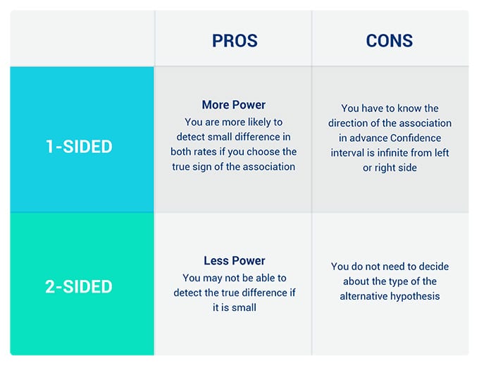
A/B test power
Not rejecting the null hypothesis does not mean that you accept it.
Again, let me state that: You never accept the null hypothesis!
If your test does not produce a statistically significant result, that only means you did not have enough evidence to reject the null hypothesis. So, it might mean that your AB test was underpowered or that the true difference between the conversion rates is very small and if you would like to detect if you need more power.
It is always a good idea to calculate the power after conducting the comparison to see if the power is not too small for a given sample size. It is even better to calculate the required sample size when planning your experiment to achieve a minimum of 80% power in your test.
When you calculate the power before planning your experiment you need to specify the minimum relevant difference that you would like to be detected. The computed sample size will be adjusted to achieve that.
The formula for the sample size calculation for the two rates comparison experiment is as follows:
For not equal variances of the two rates:
[latex]n_{C}=R\cdot n_{N}[/latex] , [latex]n_{N}[/latex] = [latex]\frac{\rho _{N}(1-\rho _{N})}{R}+\rho
_{C}(1-\rho _{C})\frac{(z_{1-\beta }+z_{1-\frac{\alpha }{2}})2^{}}{(\rho
_{N}-\rho _{C})2^{}}[/latex]
Where R is the ratio of users in a control of a new design group (equals 1 if the same number of users is assigned for both designs)
ρ is the pooled true rate (for which r was the estimator)
ß is the desired power of the study (usually 0.8 or 0.9)
[latex]\rho _{N}-\rho _{C}[/latex] is the minimal difference between the rates we would like to detect
[latex]\alpha[/latex] is the chosen significance level
It is a good idea to look how the minimal sample size for the study changes depending on the minimal difference you would like to detect in a study (effect size). The sample size increases as the effect size decreases in a nonlinear way, which is illustrated in the graph below: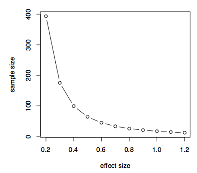
Let’s calculate the minimum sample size for our numerical example.
We assume R=1 so we want the same number of users to be assigned for the control and the variation.
Let us further assume that we want to detect 0.1 difference between the two conversion rates, the one we just observed in our sample size and we assume the same values of the true rates like the ones we observed.
Suppose we would like to have the power ß equal 0.9 and significance level [latex]\alpha[/latex] equal to 0.05 for the two-sided test.
Therefore we obtain (omitting the exact calculations):
[latex]n_{C}[/latex] = [latex]R\cdot n_{N}[/latex] , [latex]n_{N}[/latex]=[latex]\frac{\rho _{N}(1-\rho _{N})}{R}+\rho
_{C}(1-\rho _{C})\frac{(z_{1-\beta }+z_{1-\frac{\alpha }{2}})2^{}}{(\rho
_{N}-\rho _{C})2^{}}[/latex] equal to 388.
But if we change the expected rates to 0.7 and 0.85 we need only 118 users per group. That is only 18 more than we had for our samples!
Usually, the statistical software or the online calculators allow us to compute the sample size as well as the power.
Let us look at the power now.
Suppose that the alternative hypothesis is true and the difference between the rates is [latex]\theta[/latex]. Then the formula for the power for the two-sided test is as follows:
[latex]1-\beta =\phi (z-z_{1-\frac{\alpha }{2}})+\phi (-z-z_{1-\frac{\alpha
}{2}})[/latex] , where [latex]z=\frac{\rho _{N}-\rho _{C}}{\sqrt{\frac{\rho
_{N}(1-\rho _{N})}{n_{N}}+\frac{\rho _{C}(1-\rho _{C})}{n_{C}}}}[/latex]
and is the cumulative normal distribution function.
For our example, we had only 0.38 power to detect 0.1 difference between both samples equal 100 per each group. But if we change the expected rates to 0.7 and 0.9 the power increases to 0.95!
How to increase A/B test power?
Gif source: Giphy
One way of increasing a power is using a one-sided test.
Another is to increase the sample size which in case of A/B testing means increasing a traffic.
Remember that any, even very small difference between the rates could be detected if the traffic is large enough. The question is if this very small difference like 1% between the two rates is still relevant for you. In other words, can you state that the new design is better than the current one based on such a small detected difference? Kylie Vallee explains:
“Testing is supposed to make it easier for marketers to understand the impact of a certain change without the need for IT intervention, but when the difference between one-tailed and two-tailed tests goes ignored, both the marketer’s time and the IT resources are at risk of being wasted. “
Bad and good habits when it comes to one-tailed vs. two-tailed A/B tests
- Use a two-tailed test when you do not have a clue which one is a better approach for your specific situation.
- Do not conduct one after the other. If you are not able to reject the null hypothesis in 2-sided test (with less power) you will not be able to reject it with a one-tailed test (more power).
- Do not conduct 1-sided test after 2-sided. If you were able to reject the null in a two-tailed test you will be able to reject it in a one-tailed too (with the right side of the association chosen).
- Conduct a one-tailed test if your 2-tailed test was not enough powered.
- If you do not have a strong evidence that the new design is better than the current one use two-sided test to account for both possible: harmful and beneficial effects of a new design.
- Most software uses 2-sided tests but it is very easy to use them to conduct the one-sided test. In order to do it, it is enough to multiply your current significance level for the 2-sided test by [latex]2\alpha[/latex]. So, use[latex]\alpha[/latex]instead of.